Mean-Variance Portfolio Optimization When Means And Covariances Are Unknown

[Lai, Xing and Chen, 2010], in the paper “Mean-Variance Portfolio Optimization When Means And Covariances Are Unknown”, proposed a ground breaking method to do portfolio optimization. In what follows we summarize their idea and use it to implement a periodic rebalancing strategy based on the AlgoQuant framework.

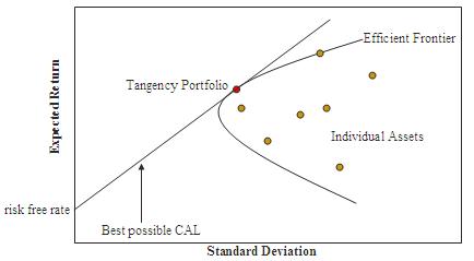
efficient frontier

Harry Markowitz won the Nobel prize for his work in mean-variance (MV) portfolio optimization in 1950s. The theory is widely regarded as fundamental in financial economics. It says, given a target return of a portfolio of m assets, the optimal (in terms of information ratio) weighting $w_{eff}$ is given by

$$w_{eff}=\arg \min_w w^T \Sigma w \text{ subject to } w^T\mu = \mu_*, w^T1 = 1$$

where $\mu$ is the expected future returns, and $\Sigma$ is the expected covariance matrix of future returns. This problem is readily solved by quadratic programming.

Nonetheless, the assumption that $\mu$ and $\Sigma$ are known in advance is very dubious. This has been referred to as the “Markowitz optimization engima”. The attempts made so far are to better forecast these estimators, namely $\hat{\mu}$ and $\hat{\Sigma}$, as accurately as possible. The maximum likelihood estimate (MLE) from the training sample is an example. It turns out, however, that MLE performs poorly because the estimators are quite different from the realized values [Michaud, 1989]. Since then, three approaches have been proposed to address the difficulty. The first approach uses a multi-factor model to reduce the dimensionality in estimating $\Sigma$ [Fan, Fan and Lv, 2008]. The second approach uses Bayes or other shrinkage estimates of $\Sigma$ [Ledoit and Wolf, 2004]. Both approaches attempt to use improved estimates of $\Sigma$ for the plug-in efficient frontier. They have also been modified to provide better estimates of $\mu$, for example, in the quasi-Bayesian approach of [Black and Litterman, 1990]. The third approach uses bootstrapping to correct for the bias of $\hat{w}_{eff}$ as an estimate of $w_{eff}.$

The innovation in [Lai, Xing and Chen, 2010] is to move away from the traditional approach of finding better estimators. They instead assume inherent uncertainty, hence risk, in these estimators. In other words, because the mean and covariance matrix of future returns are estimated from past returns, the uncertainties of these estimators should be incorporated into the portfolio risk. The authors formulate a stochastic optimization framework which solves a more fundamental problem. Given the past returns $r_1, \ldots, r_n$,

maximize $\left \{ E(w^Tr_{n+1}) - \lambda Var(w^Tr_{n+1}) \right \}$

where $w^Tr_{n+1}$ is now regarded as a random variable conditional on the past returns, and $\lambda$ is a risk-aversion index (investor’s preference).

This stochastic optimization problem is not standard due to the $E(.)^2$ term in $Var(.)$ ($Var(X) = E[X^2] - (E[X])^2$). To tackle this problem, the authors solve instead an equivalent stochastic optimization problem:

$$\max_{\eta} {E[w^T(\eta)r_{n+1}] - \lambda Var[w^T(\eta)r_{n+1}]}$$

where

$$w(\eta) = \arg \min_w {\lambda E[(w^Tr_{n+1})^2] - \eta E(w^Tr_{n+1}) }$$

and

$$\eta = 1 + 2\lambda E(W_B)$$

Next, define the function

$$C_{\lambda,\mu_n,V_n}(\eta) = E[w^T(\eta)\mu_n] + \lambda (E[w^T(\eta)\mu_n])^2 - \lambda E[w^T(\eta) V_n w(\eta)]$$

where $\mu_n$ and $V_n$ are the first and second moments of returns. The problem now becomes maximizing $C_{\lambda,\mu_n,V_n}(\eta)$ which can be achieved by any univariate maximization algorithm such as Brent’s method (BrentMinimizer in SuanShu can be used to minimize the negative of this function).

The remaining task is to estimate $\mu_n$ and $V_n$ to plug into $C_{\lambda,\mu_n,V_n}(\eta)$. $\mu_n$ can be estimated by, for example, bootstrapping, a multi-factor model, a GARCH model, etc. Similarly, $V_n = \Sigma + \mu_n \mu_n^T$ can be estimated by first estimating the sample covariance matrix $\Sigma$. As $\Sigma$ may be unstable when the sample size is small, our implementation uses a covariance-shrinkage method described in [Ledoit and Wolf 2004].

Putting all these steps together, the algorithm to compute the optimal weighting looks like this:

1. Estimate $\mu_n$ and $V_n$ from past returns
2. Estimate $a = E[w^T(\eta)\mu_n], b = E[w^T(\eta)V_nw(\eta)]$
3. Construct the univariate real function $C_{\lambda,\mu_n,V_n}(\eta) = a + \lambda a^2 - \lambda b$
4. Maximize $C_{\lambda,\mu_n,V_n}(\eta)$ over $\eta$
5. Compute the optimal weighting $w^* = w(\eta^*)$ using the optimal $\eta^*$

We have implemented this algorithm in AlgoQuant as a component/module/signal. Using our component based programming paradigm, it is easy to modify the steps in the implementation without a lot of changes to the code. For instance, we can pass in the constructor of Lai2010NPEBModel a GridSearchCetaMaximizer object instead of a BrentCetaMaximizer object to change the algorithm to maximize $C(\eta)$.

In addition, we have coded up a trading strategy using Lai’s portfolio optimization algorithm as a signal. This strategy re-balances periodically a basket of assets according to the optimal weighting computed by the model. Specifically, onDepthUpdate(), collects the returns series using the component ReturnSeries with its update() method. Then, onTimerUpdate() is triggered periodically (say, every 3 months) to call the model (passing in the returns matrix) and to send orders to re-balance the assets accordingly. We backtest this trading strategy using the Simulator object together with the historical data from Yahoo! Finance (or other data sources).

Code

• http://www.numericalmethod.com/javadoc/suanshu/com/numericalmethod/suanshu/model/lai2010/package-summary.html
• http://redmine.numericalmethod.com/projects/public/repository/svn-algoquant/show/core/src/main/java/com/numericalmethod/algoquant/model/portfoliooptimization/lai2010

References

• Black, F. and Litterman, R. (1990). Asset Allocation: Combining Investor Views with Market Equilibrium. Goldman, Sachs & Co., New York.
• Fan, J, Fan, Y and Lv, J. (2008). High dimensional covariance matrix estimation using a factor model. J. Econometrics 147 186-197.
• Lai, T. L., Xing, H. and Chen Z. (2010). Mean-variance portfolio optimization when means and covariances are unknown. Annals of Applied Statistics 2011, Vol. 5, No. 2A, p. 798-823.
• Ledoit, P. and Wolf, M. (2004). Honey, I shrunk the sample covariance matrix. J. Portfolio Management 30 110–119.
• Michaud, R. O. (1989). Efficient Asset Management. Harvard Business School Press, Boston.