Precision Is a Resource: How Much Arithmetic Does a Covariance Matrix Deserve?

The thesis of this article fits in one sentence. When we solve linear systems with a sample covariance matrix, as we do whenever we build a minimum-variance portfolio, a risk model or a regression on correlated signals, the floating-point precision we need is set by how much data we have, and not by the size or the conditioning of the problem.

We will measure this. For minimum-variance weights estimated from $T$ observations, the ratio of rounding error to estimation error behaves like $C\,u\sqrt{T}$, where $u$ is the unit roundoff and $C$ is a small constant (between about 2 and 3.5 in every experiment below in which the sample covariance is not close to singular). The condition number, which dominates every textbook error bound, cancels out of the ratio. Conditioning keeps exactly one job: it decides whether a low-precision factorization exists at all. Iterative refinement takes even that job away.

The practical consequence is blunt. Binary64 carries roughly six orders of magnitude more precision than any realistic covariance estimate can use, and a 16-bit format is enough for many everyday sample sizes.

Why ask now?

Why should anyone revisit a question that seemed settled in 1985? The IEEE 754 standard made binary64 the unremarkable default of scientific computing, and for good reason: it is cheap insurance. Very few people working in quantitative finance chose double precision; it was simply what double meant.

Two things have changed. The first is that the hardware no longer treats precisions as equal. The 2008 revision of IEEE 754 added a 16-bit binary format, the bfloat16 format has spread with machine-learning accelerators, and on such hardware lower precision is not just smaller but faster. Halving the bits halves the memory traffic, which is what usually limits dense linear algebra on large problems. Insurance that used to be free now has a premium.

The second is that numerical analysts have given us better tools to price that premium. Classical rounding error bounds grow like $nu$ and are, as Wilkinson already observed, wildly pessimistic. Higham and Mary (2019) proved that, under a model in which rounding errors are independent with zero mean, the constant can be replaced by one growing like $\sqrt{n}\,u$, with high probability. Connolly, Higham and Mary (2021) showed that stochastic rounding satisfies that model exactly, without assumptions. Carson and Higham (2018) showed how to factorize a matrix in low precision and still obtain a working-precision answer by refining in higher precision.

What is missing is an answer to the user’s question: how much precision does my problem deserve? The numerical analyst answers in terms of $\kappa(A)$. I want to argue that, for estimated matrices, this answers the wrong question.

Two errors, one answer

Let $\Sigma$ be the true covariance matrix of $n$ asset returns and $\hat\Sigma$ the sample covariance from $T$ observations. The minimum-variance weights are

$$w(\Sigma) = \frac{\Sigma^{-1}\mathbf 1}{\mathbf 1^{\top}\Sigma^{-1}\mathbf 1}.$$

What we would like is $w(\Sigma)$. What we can estimate is $w(\hat\Sigma)$. What we actually compute, in a floating-point format with unit roundoff $u$, is a third vector $\hat w$. There are therefore two errors, and they have different origins:

$$\underbrace{\frac{\lVert w(\hat\Sigma) - w(\Sigma)\rVert}{\lVert w(\Sigma)\rVert}}_{\text{statistical error}} \qquad\text{and}\qquad \underbrace{\frac{\lVert \hat w - w(\hat\Sigma)\rVert}{\lVert w(\hat\Sigma)\rVert}}_{\text{numerical error}} .$$

The first is the price of finite data and has nothing to do with computers. The second is the price of finite arithmetic and has nothing to do with data. The only sensible requirement for the second is that it be small compared with the first. Driving the numerical error down to $10^{-13}$ when the statistical error is $10^{-1}$ buys nothing: no decision changes, no risk number changes, no backtest changes. It is the computational analogue of reporting a sample mean to sixteen significant digits.

So the question is not “is the numerical error small?” but “is the numerical error small relative to the statistical error?” Asked that way, the condition number turns out to be largely beside the point.

Why the condition number cancels

Both errors are perturbations of the same matrix, and to first order they reach the weights through the same linear map. That observation is elementary, but it is the hinge of the whole argument, so it deserves a precise statement.

Proposition 1 (shared first-order operator). Let $A$ be symmetric positive definite, $x = A^{-1}\mathbf 1$ and $w = x/(\mathbf 1^{\top}x)$. For a symmetric perturbation $E$ with $\lVert A^{-1}E\rVert < 1$,

$$w(A+E) - w(A) = \mathcal L_A(E) + O(\lVert E\rVert^2), \qquad \mathcal L_A(E) = -\frac{1}{\mathbf 1^{\top}x}\,\bigl(I - w\mathbf 1^{\top}\bigr)A^{-1}E\,x .$$

Proof. From $(A+E)^{-1} = A^{-1} - A^{-1}EA^{-1} + O(\lVert E\rVert^2)$ we get $\delta x = -A^{-1}Ex + O(\lVert E\rVert^2)$. Differentiating $w = x/(\mathbf 1^{\top}x)$ gives $\delta w = (\delta x - w\,\mathbf 1^{\top}\delta x)/(\mathbf 1^{\top}x)$, and substituting proves the claim. $\square$

Now apply this with $A = \hat\Sigma$. The statistical error corresponds to $E_{\text{stat}} = \Sigma - \hat\Sigma$, since the truth is a perturbation of the estimate. A backward stable solver produces the exact solution of a nearby problem $(\hat\Sigma + E_{\text{num}})\hat x = \mathbf 1$, so the numerical error corresponds to $E_{\text{num}}$, the backward error. The ratio we care about is therefore, to first order,

$$\frac{\text{numerical error}}{\text{statistical error}} \approx \frac{\lVert\mathcal L_{\hat\Sigma}(E_{\text{num}})\rVert}{\lVert\mathcal L_{\hat\Sigma}(E_{\text{stat}})\rVert}.$$

The operator $\mathcal L_{\hat\Sigma}$ contains $\hat\Sigma^{-1}$, which is where the condition number lives. A textbook bound applies $\lVert\hat\Sigma^{-1}\rVert$ to the numerator and declares the numerical error to be of order $\kappa u$. The statistical error is amplified by the same operator. Whatever $\hat\Sigma^{-1}$ does to rounding errors, it also does to sampling errors. To the extent that the two perturbations are “generic” with respect to $\mathcal L_{\hat\Sigma}$, that is, neither is aligned with its most or least amplified directions, the amplification cancels and the ratio is governed by how large the perturbations are, not by how they are amplified.

How large are they? For the sampling perturbation there is an exact answer in the Gaussian case. If $\hat\Sigma$ is the sample covariance with estimated mean, then $(T-1)\hat\Sigma$ is Wishart with $T-1$ degrees of freedom, and

$$\operatorname{Var}\bigl(\hat\Sigma_{ij}\bigr) = \frac{\Sigma_{ij}^2 + \Sigma_{ii}\Sigma_{jj}}{T-1},$$

so every entry carries a relative error of order $T^{-1/2}$. For the rounding perturbation, the probabilistic analysis of Higham and Mary bounds the backward error of Cholesky factorization by a modest multiple of $\sqrt{n}\,u$, in the same entrywise sense, with high probability.

The cancellation argument is a heuristic, not a theorem, so we test it.

The experiment

The test is deliberately plain. We take a five-factor model with a dominant market factor, $n \in \{50, 200\}$ assets and daily scaling. We draw Gaussian returns of length $T \in \{250, 1000, 4000, 16000\}$, roughly one, four, sixteen and sixty-four years of daily data, and form the sample covariance. We compute $w(\Sigma)$ and $w(\hat\Sigma)$ in binary64, then compute $\hat w$ by Cholesky factorization and two triangular solves in emulated bfloat16 ($u = 2^{-8}$), binary16 ($u = 2^{-11}$) and binary32 ($u = 2^{-24}$). Every arithmetic result is rounded to the target significand, and every cell of the table is a median over twelve independent samples. The code is short, has no dependencies beyond numpy, and is published with this article.

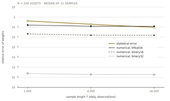Fig. 1 — Statistical error falls like $T^{-1/2}$; numerical error does not depend on $T$ at all. Where the gold line crosses a black line, that precision stops being adequate.

Figure 1 already shows the structure. The numerical error at a given precision is essentially independent of $T$, while the statistical error falls like $T^{-1/2}$. The numerical error also scales linearly with $u$: going from bfloat16 to binary16 divides it by about eight, which is $2^3$. The table makes the claim quantitative. The last three columns divide the error ratio by $u\sqrt{T}$. If the law holds, they should be roughly constant.

$n$	$T$	$\kappa(\hat\Sigma)$	statistical	ratio / $u\sqrt T$, bf16	fp16	fp32
50	250	$2.8\times10^{2}$	0.42	2.67	2.45	2.66
50	1,000	$2.1\times10^{2}$	0.21	2.13	2.26	2.35
50	4,000	$1.8\times10^{2}$	0.10	1.95	1.97	2.30
50	16,000	$1.8\times10^{2}$	0.052	1.87	2.02	2.10
200	1,000	$1.2\times10^{3}$	0.42	3.14	3.34	3.17
200	4,000	$8.1\times10^{2}$	0.19	2.58	2.66	2.66
200	16,000	$7.3\times10^{2}$	0.094	2.59	2.63	2.63
200	250	$2.0\times10^{4}$	1.54	breakdown	12.2	11.3

Across a factor of four in $n$, a factor of sixteen in $T$, a factor of seven in $\kappa$ and five orders of magnitude in $u$, the normalized ratio stays between 1.8 and 3.4. Two more regularities appear in the raw data. The statistical error lies between $0.84$ and $0.93$ times $\sqrt{n/(T-n)}$ in every configuration. The numerical error lies between $1.7$ and $3.1$ times $\sqrt{n}\,u$ in every configuration except the last. The $\sqrt n$ cancels, and what remains is $u\sqrt T$.

The last row is the exception, and it matters. With $n = 200$ and $T = 250$ the sample covariance is close to singular. Its smallest eigenvalues are pushed towards zero, in the way the Marchenko–Pastur law predicts as $n/T$ approaches one, and $\kappa(\hat\Sigma)$ jumps by a factor of twenty. Here the ratio rises to about 12: the numerical error grows to about $20\sqrt n\,u$ and starts to carry the condition number, while the statistical error still follows the same formula. In other words, the cancellation in Proposition 1 holds only while the perturbations stay generic. When $\hat\Sigma$ has eigenvalues that the data cannot resolve, rounding errors find those directions as readily as sampling errors do. Note, though, that in this regime the statistical error is 1.5: the weights are already meaningless, whatever the arithmetic.

I state the regularity as a conjecture, because I cannot prove it.

Conjecture 1 (precision–sample law). For minimum-variance weights computed by a backward stable Cholesky solve from a sample covariance of $T$ observations of $n$ assets with $n/T$ bounded away from one, the ratio of numerical to statistical error satisfies

$$\frac{\lVert\hat w - w(\hat\Sigma)\rVert}{\lVert w(\hat\Sigma) - w(\Sigma)\rVert} \asymp u\sqrt{T},$$

with constants depending only weakly on the factor structure and not on $\kappa(\hat\Sigma)$.

What would a proof need? It would need a version of the Higham–Mary bound for the forward error in the direction that $\mathcal L_{\hat\Sigma}$ cares about, together with a lower bound on the statistical error in the same direction. The second is classical random matrix theory. The first is, as far as I know, open, because probabilistic rounding error analyses have so far been written for backward error and for generic forward error, not for the forward error of a statistic.

A budget in bits

If the law holds, choosing a precision becomes arithmetic. Suppose we want the numerical error to be at most a fraction $\rho$ of the statistical error. With $u = 2^{-t}$ for a $t$-bit significand and a constant $C \approx 3$, we need

$$t \;\ge\; \log_2\!\frac{C\sqrt T}{\rho}.$$

The table below evaluates this for daily data.

history	$T$	bits for $\rho = 10\%$	bits for $\rho = 1\%$
1 year	250	8.9	12.2
4 years	1,000	9.9	13.2
16 years	4,000	10.9	14.2
64 years	16,000	11.9	15.2

Binary32 has 24 bits. By the same formula it would remain within 1% of the statistical error until $T$ reached about $3\times10^{9}$ observations, which is twelve million years of daily data, or several years of tick data for a liquid instrument. Binary64 has 53 bits. The twenty-nine extra bits are not protecting your answer from anything.

Binary16, with 11 bits, is adequate at the 10% level up to about sixteen years of daily data and within 20% beyond that. Bfloat16, with 8 bits, is not adequate at the 10% level for any history in the table. Figure 1 shows exactly this: the bfloat16 line meets the statistical error near $T = 16{,}000$, and the binary16 line stays below it by a factor of six or more.

Conditioning decides existence, not accuracy

Does the condition number then play no role? It does play one, but a different one. A low-precision Cholesky factorization can fail. When $\kappa u$ is large, rounding can make a pivot non-positive and the factorization breaks down. A classical sufficient condition due to Demmel guarantees success when a modest multiple of $n^{3/2}\kappa_2(H)u$ is below one, where $H$ is the matrix scaled to unit diagonal (Higham 2002, ch. 10). In our experiments bfloat16 broke down in all twelve samples with $n = 200$, $T = 250$, where $\kappa u \approx 80$. Binary16 survived there with $\kappa u \approx 10$, which shows how conservative the sufficient condition is.

So conditioning determines whether you can factorize at all in a given precision. And once the factorization exists, even a poor low-precision factor can be turned into an accurate solve. In classical iterative refinement we keep the low-precision factor $\hat L$, compute residuals $r = b - A\hat x$ in binary64, solve $\hat L\hat L^{\top}d = r$ with the cheap factor, and update $\hat x \leftarrow \hat x + d$. Carson and Higham (2018) analyse this, and its three-precision generalizations, in detail. The informal summary is that each step multiplies the error by a factor of order $\kappa u_f$, where $u_f$ is the factorization precision, until the error reaches the accuracy the residual precision allows.

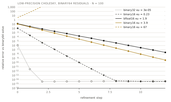Fig. 2 — Refinement with a low-precision Cholesky factor and binary64 residuals ($n = 100$, $T = 1000$). The contraction factor per step is about $0.05$–$0.13\times\kappa u$.

Figure 2 shows the textbook picture with real numbers. A binary32 factor gives binary64 accuracy within two to four steps at every condition number we tried, up to $\kappa = 7\times10^{5}$. A binary16 factor with $\kappa u = 0.23$ contracts the error by a factor of about $0.02$ per step. A bfloat16 factor with $\kappa u = 1.9$, which by the usual rule should not work at all, still contracts by about $0.25$ per step. Binary16 with $\kappa u = 3.9$ contracts by $0.2$. At $\kappa u = 67$ the iteration diverges, as it must.

Put the two results together and the division of labour is clean. The data decides how many bits the answer deserves, which is Conjecture 1. The conditioning decides how many bits the factorization needs, which is at most $\log_2\kappa$ plus a few. Refinement connects the two, so the expensive $O(n^3)$ work happens in the precision the conditioning requires and only the $O(n^2)$ residual work happens in higher precision. In no case is binary64 needed for the factorization of an estimated covariance matrix of modest condition.

A different regime: long sums

Not every computation in finance is a linear solve. Many are accumulations: a profit-and-loss series summed over years, a Monte Carlo estimator averaged over millions of paths, an exponentially weighted statistic updated tick by tick. Here the relevant count is not the sample size but the number of operations, and round-to-nearest has a failure mode that no amount of data fixes.

Accumulate $N$ positive increments of size about $10^{-3}$ in a format with an 11-bit significand. Once the running sum $\hat s$ exceeds roughly $x/u$, each new increment is smaller than half the spacing of the floating-point numbers near $\hat s$, and round-to-nearest returns $\hat s$ unchanged. The sum stagnates. In our run it stalls near 4 while the true sum climbs to 262, an error of 98% (Figure 3). This is not a rare corner case. It is what happens to any long accumulation in low precision, and it is the reason compensated summation (Kahan 1965) and pairwise summation exist.

Stochastic rounding behaves completely differently. It rounds $y$ up to the next representable number with probability equal to its fractional distance from the number below, so $\mathbb E[\operatorname{fl}(y)] = y$. Connolly, Higham and Mary (2021) showed that this makes the rounding errors mean independent and that the $\sqrt n\,u$ backward error bounds then hold without further assumptions. For accumulations of positive terms we can say something sharper, and the argument is short enough to give in full.

Theorem 2 (stochastic rounding does not drift). Let $x_1, \dots, x_N \ge 0$ be representable numbers with exact partial sums $s_k$ and total $S = s_N$. Let $\hat s_0 = 0$ and $\hat s_k = \operatorname{fl}_{\mathrm{SR}}(\hat s_{k-1} + x_k)$ with a $t$-bit significand, and put $u = 2^{-t}$. Then $\mathbb E[\hat s_N] = S$ and

$$\mathbb E\bigl[(\hat s_N - S)^2\bigr] \;\le\; u\Bigl(S^2 + \sum_{k=1}^{N}x_k^2\Bigr) + R,$$

where the remainder $R$ comes only from the at most $B = \lceil\log_2(S/x_{\min})\rceil + 1$ steps at which the sum enters a new binade, and satisfies $R \le (1+o(1))\,B\,u^2S^2$. In particular the relative root-mean-square error is at most $\sqrt u\,(1 + o(1))$, independently of $N$.

Proof. Write $y_k = \hat s_{k-1} + x_k$ and $\varepsilon_k = \hat s_k - y_k$, so that $\hat s_N - S = \sum_k \varepsilon_k$. Let $\mathcal F_{k}$ be the history up to step $k$. Stochastic rounding gives $\mathbb E[\varepsilon_k \mid \mathcal F_{k-1}] = 0$, so the errors form a martingale difference sequence. Hence $\mathbb E[\hat s_N] = S$, and since cross terms vanish, $\mathbb E[(\hat s_N - S)^2] = \sum_k \mathbb E[\operatorname{Var}(\varepsilon_k \mid \mathcal F_{k-1})]$.

Let $\Delta_k$ be the spacing of $t$-bit numbers at $y_k$, so that $\Delta_k \le 2u\,y_k$, and let $d_k$ be the distance from $y_k$ down to the nearest representable number. Rounding up has probability $d_k/\Delta_k$, so $\operatorname{Var}(\varepsilon_k \mid \mathcal F_{k-1}) = d_k(\Delta_k - d_k) \le \Delta_k d_k$. If $\hat s_{k-1}$ lies on the grid of spacing $\Delta_k$, which is the case unless $y_k$ has just crossed into a coarser binade, then $d_k = x_k \bmod \Delta_k \le x_k$. Therefore $\operatorname{Var}(\varepsilon_k\mid\mathcal F_{k-1}) \le 2u\,x_k\,y_k$. Taking expectations, and using unbiasedness, $\mathbb E[y_k] = \mathbb E[\hat s_{k-1}] + x_k = s_k$, so

$$\sum_k \mathbb E\bigl[\operatorname{Var}(\varepsilon_k\mid\mathcal F_{k-1})\bigr] \;\le\; 2u\sum_k x_k s_k \;=\; u\Bigl(S^2 + \sum_k x_k^2\Bigr),$$

by the identity $2\sum_k x_k s_k = S^2 + \sum_k x_k^2$. At the at most $B$ binade crossings we use only $\operatorname{Var} \le \Delta_k^2/4 \le u^2 y_k^2$. Since $\mathbb E[y_k^2] = s_k^2 + \operatorname{Var}(\hat s_{k-1}) \le S^2(1 + O(u))$ by what has already been shown, $R \le (1+o(1))\,B\,u^2 S^2$. $\square$

The proof contains the reason the result holds. The variance of a stochastic rounding is not of order $u^2y^2$, as a naive bound would suggest, but of order $u\,x\,y$: it is proportional to the increment, because a small increment is rounded up only rarely. The variances therefore add up to a multiple of $\sum x_k s_k$, which is of order $S^2$, instead of growing with $N$.

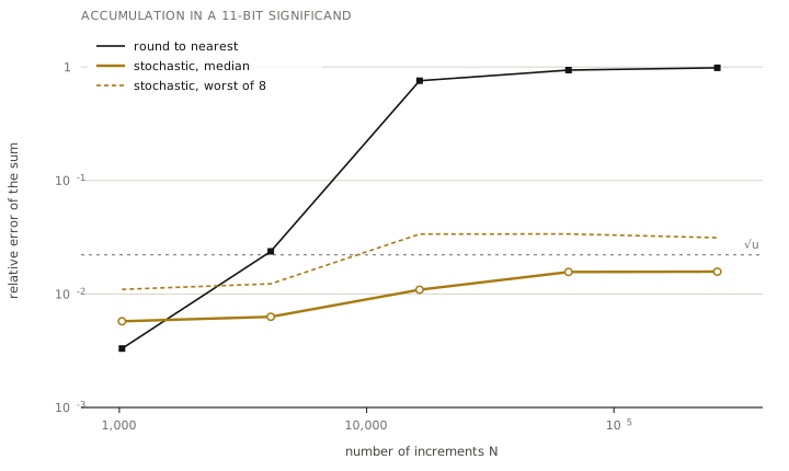Fig. 3 — Summing $N$ increments of about $10^{-3}$ with an 11-bit significand. Round-to-nearest stagnates; stochastic rounding saturates below $\sqrt u$, as Theorem 2 predicts.

Figure 3 is the experiment. With $u = 2^{-11}$, Theorem 2 bounds the relative RMS error by $\sqrt u \approx 0.022$, which predicts a median absolute error of about $0.674\sqrt u \approx 0.015$. The observed median over eight runs at $N = 2^{18}$ is $0.016$, consistent with the bound to within the sampling error of eight runs, and it barely moves between $N = 2^{16}$ and $N = 2^{18}$.

Note the contrast with the linear solve. There, the data set the budget and $N$ played no role. Here, $N$ is the enemy of round-to-nearest, and the rounding mode, not the number of bits, is the cure.

What changes on Monday

If you build risk models, three things follow.

First, use binary32 for covariance linear algebra by default, and treat binary64 as something that has to be justified, for example by $n/T$ close to one, by extreme conditioning, or by a downstream computation that genuinely needs it. The justification “the answer must be accurate” does not count, because the answer was never more accurate than $T^{-1/2}$.

Second, make precision a function of history length. A model estimated on two years of daily data cannot benefit from more than about thirteen bits in its solve. If the hardware you run on is faster at 16 bits, the budget formula tells you when you may use it. Iterative refinement with binary64 residuals is the safety net when the conditioning objects.

Third, treat accumulations separately. A sum over millions of terms is not protected by statistics. Use pairwise or compensated summation, or stochastic rounding where it is available, and do not let a low-precision accumulator run unattended.

What this does not show

The law in Conjecture 1 is empirical and was measured on one family of synthetic markets: Gaussian returns from a stationary five-factor model. Real returns are heavy-tailed and non-stationary. Both effects increase the statistical error, which should only strengthen the conclusion, but that is an expectation, not a measurement.

The experiments emulate the significand of each format, not its exponent range. That omission matters in practice: daily variances are of order $10^{-4}$ to $10^{-6}$, and binary16’s smallest normal number is about $6\times10^{-5}$. Anyone who actually computes in binary16 must rescale, for example by working with correlations or with returns in basis points, and must check for underflow.

Only the plain sample covariance and the minimum-variance portfolio were studied. Shrinkage estimators such as that of Ledoit and Wolf (2004) reduce both the statistical error and the condition number. How they move the constant $C$ is an open question, and so is the behaviour of the ratio for mean-variance portfolios, which add the much larger estimation error of expected returns, the effect Michaud (1989) called the optimization enigma.

Nothing here measures speed. The argument is about how many bits the answer deserves, not about how fast a given machine delivers them.

Finally, the cancellation of the condition number is supported by Proposition 1 and by the measurements, but it is not proved. It fails where it should, as $n/T \to 1$. A proof would need a probabilistic forward error analysis directed at a statistic rather than at the solution vector as a whole, which I believe is the most interesting open problem this article leaves behind.

References

• Carson, E. and Higham, N. J. (2018). Accelerating the solution of linear systems by iterative refinement in three precisions. SIAM Journal on Scientific Computing, 40(2), A817–A847.
• Connolly, M. P., Higham, N. J. and Mary, T. (2021). Stochastic rounding and its probabilistic backward error analysis. SIAM Journal on Scientific Computing, 43(1), A566–A585.
• Higham, N. J. (2002). Accuracy and Stability of Numerical Algorithms, 2nd ed. SIAM.
• Higham, N. J. and Mary, T. (2019). A new approach to probabilistic rounding error analysis. SIAM Journal on Scientific Computing, 41(5), A2815–A2835.
• Kahan, W. (1965). Further remarks on reducing truncation errors. Communications of the ACM, 8(1), 40.
• Ledoit, O. and Wolf, M. (2004). A well-conditioned estimator for large-dimensional covariance matrices. Journal of Multivariate Analysis, 88(2), 365–411.
• Michaud, R. O. (1989). The Markowitz optimization enigma: is “optimized” optimal? Financial Analysts Journal, 45(1), 31–42.
• Wilkinson, J. H. (1963). Rounding Errors in Algebraic Processes. Prentice-Hall.

Code and data. All numbers and figures in this article come from experiments.py (Python 3.9, numpy 2.0), which runs in under a minute on a laptop and writes results.json. Random seeds are fixed.