Training Is Numerical Integration: What Numerical Analysis Says About Learning Rates

Here is the thesis. Gradient descent is a numerical method for an ordinary differential equation, and the most useful things we know about training follow from taking that literally. The learning rate is not a speed setting. It is a choice of model, because a gradient descent run with step $h$ follows, with error $O(h^2)$, the exact gradient flow of a different loss, $L + \tfrac h4\lVert\nabla L\rVert^2$. And the number of steps is not a budget. Together with the step size, it defines a training time $t = kh$, and for least-squares problems that training time is, up to a constant factor in risk, the inverse of a ridge penalty.

None of the ingredients is new. Backward error analysis is half a century old, the modified loss was written down by Barrett and Dherin (2021), and the link between early stopping and ridge regression is classical. What I want to show is that, put together, they turn the learning rate, the step count and the regularization strength from three dials into one. They also explain why, in return prediction, early stopping is shrinkage, and they tell us which experiments not to bother running.

The phenomenon everyone has seen

What does every practitioner who has trained a model know? Three things, usually learned the hard way.

First, there is a largest learning rate beyond which training diverges, and good runs often sit not far below it. Second, if you never stop, a flexible model will eventually fit the noise. Training error keeps falling while test error turns around and climbs. Third, the learning rate and the number of epochs interact: halve one and you often need to double the other to get the same result, but not always, and the cases where the rule fails are where the interesting behaviour lives.

Each of these facts is usually explained separately, with a different vocabulary: optimization for the first, statistics for the second, folklore for the third. A numerical analyst sees one object behind all three: a one-step method for an ODE, with a stability limit, a modified equation and a time variable.

Gradient descent is the forward Euler method

Gradient descent with step $h$,

$$\theta_{k+1} = \theta_k - h\,\nabla L(\theta_k),$$

is precisely the forward Euler method applied to the gradient flow

$$\dot\theta(t) = -\nabla L(\theta(t)).$$

Iterate $k$ approximates the flow at time $t = kh$. The flow itself is the idealized learner. It has no step size, it decreases $L$ monotonically, and for convex problems it converges to a minimizer. Everything a real run does differently from the flow is a discretization effect, and numerical analysis has spent sixty years classifying discretization effects.

The first is stability. Near a minimum, $L$ is approximately quadratic with Hessian $H$. In an eigendirection of $H$ with eigenvalue $\lambda$, one Euler step multiplies the deviation from the minimum by $1 - h\lambda$.

Proposition 1 (stability limit). For a quadratic loss with Hessian $H \succeq 0$, gradient descent converges for every starting point if and only if $0 < h < 2/\lambda_{\max}(H)$ (with $\lambda_{\max} > 0$). For $1/\lambda_{\max} < h < 2/\lambda_{\max}$ the component along the top eigenvector converges with alternating sign.

Proof. The error $e_k = \theta_k - \theta^\star$ satisfies $e_{k+1} = (I - hH)e_k$, so each eigencomponent is multiplied by $1 - h\lambda_i$ per step. All components converge if and only if $\lvert 1 - h\lambda_i\rvert < 1$ for every $\lambda_i > 0$, that is, $h < 2/\lambda_{\max}$. The sign of $1 - h\lambda_{\max}$ is negative exactly when $h > 1/\lambda_{\max}$. $\square$

This is the textbook stability region of the forward Euler method, restated in the vocabulary of machine learning. The “largest learning rate” is $2/\lambda_{\max}$, and $\lambda_{\max}$, the sharpness of the loss, plays the role that the stiffest eigenvalue plays for a differential equation. That observation sounds trivial. Its consequences are not, because for neural networks $\lambda_{\max}$ is not a constant: training changes it. We will return to this.

The learning rate chooses the loss

The second effect is subtler and more important. A numerical method does not solve the equation you gave it. To higher order, it solves a nearby equation exactly. This is the idea behind backward error analysis for differential equations, developed at length by Hairer, Lubich and Wanner (2006). Find the modified vector field whose exact flow passes through the numerical iterates, and you know what the method is really doing.

For gradient descent the computation is short. We look for a vector field $f_h = -\nabla L + h f_1$ whose exact flow over a time $h$ agrees with one Euler step up to $O(h^3)$.

Proposition 2 (modified loss; Barrett and Dherin 2021). Let $L$ be three times continuously differentiable. The flow of

$$\dot\theta = -\nabla \widetilde L_h(\theta), \qquad \widetilde L_h = L + \frac h4\,\lVert\nabla L\rVert^2,$$

agrees with one step of gradient descent with step $h$ up to $O(h^3)$. Consequently, over any fixed time interval $[0, t]$ the gradient descent iterates stay within $O(h^2)$ of this flow, whereas they are only $O(h)$ from the gradient flow of $L$ itself.

Derivation. Write $g = \nabla L$ and $H = \nabla^2 L$, and expand the flow of $\dot\theta = f(\theta)$ with $f = -g + hf_1$ in powers of the elapsed time $h$:

$$\theta(h) = \theta + h f + \tfrac{h^2}{2}\,f'f + O(h^3) = \theta - hg + h^2\bigl(f_1 + \tfrac12 Hg\bigr) + O(h^3),$$

where we used $f'f = (-H)(-g) + O(h) = Hg + O(h)$. Matching this with the Euler step $\theta - hg$ requires $f_1 = -\tfrac12 Hg$. Since $\nabla\bigl(\tfrac12\lVert g\rVert^2\bigr) = Hg$, we have $f_1 = -\nabla\bigl(\tfrac14\lVert g\rVert^2\bigr)$, and therefore $f = -\nabla\bigl(L + \tfrac h4\lVert\nabla L\rVert^2\bigr)$. The global statement follows from the local one by the standard argument: a local error of $O(h^3)$ accumulated over $t/h$ steps of a Lipschitz flow gives a global error of $O(h^2)$. $\square$

Read the modified loss as a statement about learning. Gradient descent with step $h$ does not minimize $L$. It minimizes $L$ plus a penalty on the squared gradient norm, with a weight proportional to the learning rate. Trajectories through regions where the loss is steep are penalized. A larger learning rate is therefore not “the same optimization, faster”. It is a different objective, with a stronger preference for flat regions. Barrett and Dherin call this implicit gradient regularization, and Smith, Dherin, Barrett and De (2021) extended the analysis to stochastic gradient descent, where minibatch noise contributes a further penalty.

The quadratic case shows that nothing has been lost in the expansion. For $L(\theta) = \tfrac12\theta^{\top}A\theta$ the modified loss is $\widetilde L_h = \tfrac12\theta^{\top}\bigl(A + \tfrac h2A^2\bigr)\theta$, so the modified flow contracts an eigendirection with eigenvalue $s$ at the rate $s(1 + \tfrac{hs}{2})$. Over one step of length $h$ that is a factor $\exp\bigl(-hs - \tfrac{h^2s^2}{2}\bigr)$. Gradient descent multiplies by $1 - hs = \exp\bigl(\ln(1-hs)\bigr) = \exp\bigl(-hs - \tfrac{h^2s^2}{2} - \tfrac{h^3s^3}{3} - \cdots\bigr)$. The two agree through second order and differ at third order, exactly as Proposition 2 says. The same expansion shows where the description must fail: the series for $\ln(1-hs)$ diverges as $hs \to 1$, and for $hs > 1$ the factor $1 - hs$ is negative, which no exponential can reproduce. The modified equation lives inside the stability region, and loses its meaning at the halfway point to the edge.

Is the $O(h^2)$ claim true in practice, outside the asymptotic regime? We can check directly. Take a one-hidden-layer tanh network with 48 parameters, fitted to 64 points of a smooth function. Run gradient descent to time $t = 2$ with five learning rates, and integrate both the gradient flow and the modified flow to high accuracy with a fourth-order Runge–Kutta method. The code computes Hessian–gradient products by differencing the analytic gradient.

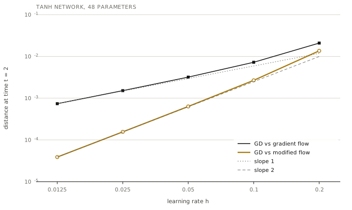Fig. 1 — Gradient descent is first-order close to the gradient flow of $L$ and second-order close to the flow of $L + \tfrac h4\lVert\nabla L\rVert^2$.

Halving $h$ halves the distance to the gradient flow, with successive ratios $2.88, 2.27, 2.11, 2.05$, and quarters the distance to the modified flow, with ratios $5.08, 4.23, 4.06, 4.02$. At $h = 0.0125$ the modified flow is nineteen times closer to what gradient descent actually did. Even for a small non-convex network, the modified loss is not a metaphor. It is a quantitatively better description of the training run than the loss we wrote down.

Training time is a regularization parameter

The third effect concerns the time variable. In the flow picture, a training run is parameterized not by its number of steps $k$ but by the time $t = kh$ it has integrated. For least squares this can be made exact, and the result shows directly what training time does.

Let $A = X^{\top}X/n$ be the sample covariance of the features, with eigenpairs $(s_i, v_i)$, and let $b = X^{\top}y/n$. The least-squares loss is $L(w) = \tfrac12 w^{\top}Aw - b^{\top}w + \text{const}$, and its minimizer, ordinary least squares, has component $b_i/s_i$ along $v_i$, writing $b_i = v_i^{\top}b$.

Proposition 3 (training as a spectral filter). Started from $w_0 = 0$, each of the following estimators has component $\varphi(s_i)\,b_i/s_i$ along $v_i$, with

$$\begin{aligned} &\text{gradient descent after } k \text{ steps:} && \varphi^{\mathrm{GD}}_{k}(s) = 1 - (1-hs)^k,\\ &\text{gradient flow at time } t: && \varphi^{\mathrm{GF}}_{t}(s) = 1 - e^{-ts},\\ &\text{ridge regression with penalty } \alpha: && \varphi^{\mathrm{R}}_{\alpha}(s) = \frac{s}{s+\alpha}. \end{aligned}$$

Proof. Gradient descent gives $w_{k+1} = (I - hA)w_k + hb$. Along $v_i$ this is the scalar recursion $c_{k+1} = (1 - hs_i)c_k + hb_i$ with $c_0 = 0$, whose solution is $c_k = \bigl(1 - (1-hs_i)^k\bigr)b_i/s_i$. The flow $\dot w = b - Aw$ gives $c(t) = (1 - e^{-ts_i})b_i/s_i$. Ridge regression solves $(A + \alpha I)w = b$, so $c = b_i/(s_i + \alpha)$. $\square$

The filter $\varphi$ is the fraction of each direction that the estimator has learned. Directions with large eigenvalues, the strong and stable patterns in the data, are learned early. Directions with small eigenvalues, where the sample covariance is mostly noise, are learned late, and their components $b_i/s_i$ are exactly the ones that blow up in ordinary least squares. Stopping at time $t$ keeps the first and suppresses the second. That is what shrinkage is.

None of this was discovered by machine learning. In 1951 Landweber proposed solving integral equations of the first kind, the model of an ill-posed inverse problem, by exactly the iteration $w_{k+1} = w_k + h\,X^{\top}(y - Xw_k)$, which is gradient descent on least squares. The numerical analysts who studied it found the behaviour of Figure 3 below decades before anyone drew a validation curve. The iterates first approach a sensible regularized solution and then, as the iteration starts to resolve the noise-dominated small singular values, move away from it again. They called this semiconvergence, and they treated the iteration count as a regularization parameter, to be chosen by a stopping rule such as Morozov’s discrepancy principle. The theory of iterative regularization that grew from it is set out in the monograph of Engl, Hanke and Neubauer (1996). Early stopping in neural network training is the same phenomenon, met again by a different community with a different vocabulary. Proposition 3 is, for an inverse-problems theorist, the starting point rather than the conclusion.

The reason this history matters is not priority. The inverse-problems literature asks a question that machine learning has mostly not asked: how should the stopping index depend on the noise level? Its answer, for a range of smoothness assumptions on the truth, is a precise rate. That is a quantitative prediction about training time that can be tested in finance, where the noise level of returns is large, roughly known, and changes over time.

How close are the three filters? Two inequalities answer that, and both are short to prove.

Proposition 4. (a) If $h\lambda_{\max}(A) \le \tfrac12$ and $t = kh$, then

$$\sup_{0 \le s \le \lambda_{\max}}\bigl\lvert\varphi^{\mathrm{GD}}_k(s) - \varphi^{\mathrm{GF}}_t(s)\bigr\rvert \;\le\; \frac{h\lambda_{\max}}{e}.$$

(b) With $\alpha = 1/t$,

$$\sup_{s \ge 0}\bigl\lvert\varphi^{\mathrm{GF}}_t(s) - \varphi^{\mathrm{R}}_{1/t}(s)\bigr\rvert = \max_{z \ge 0}\Bigl(1 - e^{-z} - \frac{z}{1+z}\Bigr) \approx 0.2036,$$

attained at $z = ts \approx 2.51$.

Proof. (a) Put $x = hs \in [0, \tfrac12]$. Since $\ln(1-x) = -x - x^2\bigl(\tfrac12 + \tfrac x3 + \tfrac{x^2}4 + \cdots\bigr) \ge -x - x^2$ for $x \le \tfrac12$, we have $e^{-kx} \ge (1-x)^k \ge e^{-kx}e^{-kx^2}$. Hence

$$0 \le \varphi^{\mathrm{GD}}_k - \varphi^{\mathrm{GF}}_t = e^{-kx} - (1-x)^k \le e^{-kx}\bigl(1 - e^{-kx^2}\bigr) \le (kx)e^{-kx}\cdot x \le \frac{x}{e},$$

using $1 - e^{-y} \le y$ and $ye^{-y} \le 1/e$. (b) Both filters depend on $s$ only through $z = ts$, and the difference is a function of one variable, which is non-negative and vanishes at $0$ and at infinity. Its maximum is found numerically. $\square$

The filters, computed exactly, are shown in Figure 2. With $h\lambda_{\max} = 0.2$ the largest gap between gradient descent and gradient flow is $0.0054$, well inside the bound $0.074$ of part (a). With $h\lambda_{\max} = 1.0$ it is $0.028$. With $h\lambda_{\max} = 1.9$, close to the stability limit, the gradient descent filter overshoots to $1.59$ in the stiffest direction, which is the alternating-sign regime of Proposition 1. The gap between gradient flow and ridge is $0.2036$ in every case, as part (b) says.

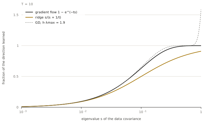Fig. 2 — The three spectral filters at $t = 10$. Early stopping and ridge regression differ by at most $0.21$ in any direction. Gradient descent tracks the flow until the step size approaches the stability limit.

A filter gap of $0.2$ is a statement about each direction separately. For the statistical question, how good the estimator is, Ali, Kolter and Tibshirani (2019) proved the stronger and more useful result. Under weak assumptions, and with no assumptions on the feature matrix, the estimation risk of gradient flow at time $t$ is within a factor of $1.69$ of the risk of ridge regression with $\alpha = 1/t$, for every $t$. Early stopping does not merely resemble ridge regression. It is ridge regression up to a constant factor in risk.

What this means for return prediction

Return prediction is close to the worst case for the methods above, and therefore the best case for the argument. The signals are many and individually weak, the samples are short, the features are correlated, and the noise is large. Ordinary least squares is hopeless in that setting, and everyone knows it. What is less often noticed is that “I trained a model with gradient descent and stopped when the validation error was lowest” and “I fitted a ridge regression and chose the penalty by validation” are, by Proposition 3, nearly the same procedure.

The experiment makes this concrete. We take 200 correlated synthetic signals with weak true coefficients, 300 training days and 5,000 test days, and fit linear predictors by gradient descent from zero at three learning rates: $h\lambda_{\max} = 0.2$, $1.0$ and $1.9$.

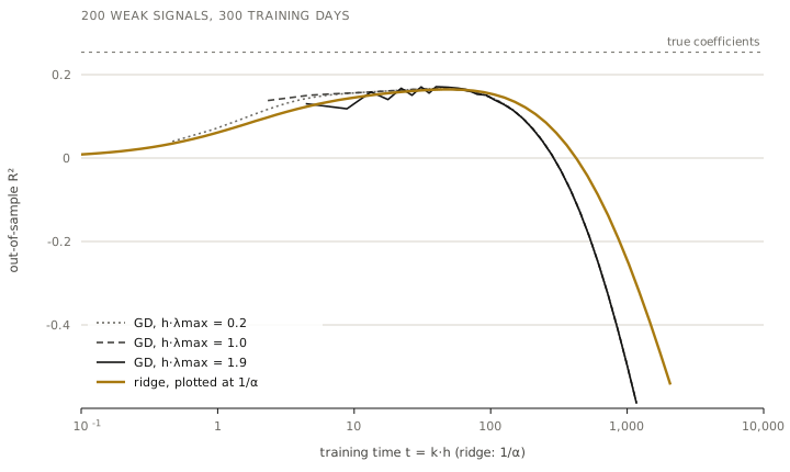Fig. 3 — Out-of-sample $R^2$ along the training path, for three learning rates, plotted against training time $t = kh$. Ridge regression is plotted against $1/\alpha$. The vertical axis is truncated at $-0.6$; ordinary least squares reaches $-1.79$.

Plotted against the number of steps, the three gradient descent runs would look like three different experiments, since one takes almost ten times as many steps as another. Plotted against training time, they are one curve. The best out-of-sample $R^2$ is $0.1662$ at $t = 40.5$ for $h\lambda_{\max} = 0.2$, $0.1662$ at $t = 41.9$ for $h\lambda_{\max} = 1.0$, and $0.1709$ at $t = 39.8$ for $h\lambda_{\max} = 1.9$. Ridge regression at $\alpha = 1/40$ gives $0.1640$, and its best value over all penalties is $0.1645$. Ordinary least squares, the end point of every one of these paths, gives $-1.79$ on the test set while explaining 74% of the training variance. For reference, the true coefficients would give $0.2536$.

Proposition 3 also lets us say how complex the stopped model is. Ridge regression has a standard measure of effective model size, its degrees of freedom $\operatorname{df}(\alpha) = \sum_i s_i/(s_i + \alpha)$, the trace of the matrix that maps observations to fitted values. The same trace for gradient flow is $\operatorname{df}(t) = \sum_i \bigl(1 - e^{-ts_i}\bigr)$, the sum of the filter over all directions. At the best stopping time in our experiment, $t = 40.5$, this gives $\operatorname{df} = 38.1$. At the best ridge penalty it gives $40.8$. The model has 200 coefficients, but the predictor that works best uses about forty effective parameters, and the remaining 160 directions are mostly suppressed. Ordinary least squares uses all 200, and that is precisely why it fails.

This is a useful way to talk about trading models. “We trained for 40 units of time” means little to a risk committee. “The model has about forty effective parameters, estimated from 300 observations” is a sentence everyone in the room can evaluate. And the number comes free with the spectral decomposition of the feature covariance.

Three practical rules follow.

The first is to report training time, not steps or learning rate. The pair $(h, k)$ is a redundant parameterization of $t = kh$ whenever $h\lambda_{\max}$ is comfortably below one. A grid search over learning rates and epochs mostly searches the same one-dimensional family twice. Search over $t$, keep $h$ below the stability limit, and spend the saved compute on validating $t$ honestly, for example out of time.

The second is to treat the stopping time with the same suspicion as a shrinkage intensity. It is a regularization parameter fitted to data, and choosing it on the same sample that measures performance is exactly as optimistic as choosing a ridge penalty that way. The literature on overfitting in strategy optimization applies to it without change.

The third is to look at the loss you are really minimizing. With a non-trivial learning rate, the objective is $L + \tfrac h4\lVert\nabla L\rVert^2$, which prefers parameter regions where the fitted model is insensitive to its parameters. For a trading model that is often a desirable property. But it is a modelling choice, and it is being made by the learning rate, usually without anyone noticing.

What the numerical analyst predicts

A framework is worth something only if it predicts. Here are three predictions, stated so that they can fail.

Collapse. For problems that are approximately quadratic near their minimizers, test performance along a training path should depend on $(h, k)$ only through $t = kh$, up to corrections of order $h\lambda_{\max}$. Figure 3 confirms this for linear models. For deep networks it is a hypothesis, and the obvious test is to replot published learning-rate sweeps against $t$.

Order. Any modification of gradient descent that raises its order as an integrator, such as extrapolation or Runge–Kutta-type updates, also removes the $\tfrac h4\lVert\nabla L\rVert^2$ term from the modified loss. Such methods should therefore lose some of the implicit regularization of plain gradient descent, and a careful comparison should find them slightly worse in out-of-sample performance at equal training loss, unless the lost regularization is added back explicitly. This is a heuristic consequence of Proposition 2, not a theorem about generalization.

Noise. The theory of iterative regularization says that the optimal stopping time should shrink as the noise level grows, at a rate fixed by how smooth the truth is relative to the data covariance. Translated to finance: the same model on the same signals should be stopped earlier in volatile regimes than in calm ones, and a fixed number of epochs carried across regimes is systematically mis-regularized in at least one of them. This is directly testable on any return-prediction pipeline that is retrained on a rolling window, by recording the validated stopping time together with the realized volatility of the training window. I have not run that test, and the synthetic experiment above, which has a single fixed noise level, cannot.

Stiffness. Because the learning rate fixes the stability limit $2/h$, any training dynamics that increase the sharpness $\lambda_{\max}$ must eventually collide with that limit. Cohen, Kaur, Li, Kolter and Talwalkar (2021) observed exactly such a collision empirically: in full-batch training of neural networks, the sharpness rises until it hovers just above $2/h$, while the loss keeps decreasing non-monotonically. In the language of this article, the network trains at the edge of the stability region of the forward Euler method. Why it can keep doing so without diverging is not explained by the arguments above.

What this does not show

The modified-equation argument is asymptotic in the step size. It is accurate when $h\lambda_{\max}$ is small, it is informative when $h\lambda_{\max}$ is of order one, and it says nothing reliable at the edge of stability, which is where Cohen et al. find practical training. The most interesting regime of modern training is precisely the one in which the clean picture of this article breaks down, and a theory of it is, as far as I know, still incomplete.

The equivalence between early stopping and ridge regression is exact only for least squares. For neural networks it holds locally, around a point where the loss is approximately quadratic, and the relevant matrix $A$ is then a changing Hessian, not a fixed covariance.

Stochastic gradient descent adds noise to the integrator. Its modified loss contains further terms (Smith et al. 2021), and its continuous-time limit is a stochastic differential equation rather than an ODE (Li, Tai and E 2017). None of the experiments here used minibatches.

The experiments are small by design: a 48-parameter network and a 200-feature linear model, both chosen so that every number can be reproduced on a laptop in seconds. They test the mathematics. They do not establish how large the effects are in large models, and nothing here should be read as a claim about any particular system.

Finally, the finance example uses synthetic data with stationary, Gaussian noise and a known truth. Real return prediction adds non-stationarity, which makes any fixed stopping time stale, and that is an argument for re-validating $t$ out of time, not against the framework.

References

• Ali, A., Kolter, J. Z. and Tibshirani, R. J. (2019). A continuous-time view of early stopping for least squares regression. Proceedings of AISTATS, PMLR 89, 1370–1378.
• Barrett, D. G. T. and Dherin, B. (2021). Implicit gradient regularization. International Conference on Learning Representations (ICLR).
• Cohen, J. M., Kaur, S., Li, Y., Kolter, J. Z. and Talwalkar, A. (2021). Gradient descent on neural networks typically occurs at the edge of stability. International Conference on Learning Representations (ICLR).
• Engl, H. W., Hanke, M. and Neubauer, A. (1996). Regularization of Inverse Problems. Kluwer Academic Publishers.
• Hairer, E., Lubich, C. and Wanner, G. (2006). Geometric Numerical Integration: Structure-Preserving Algorithms for Ordinary Differential Equations, 2nd ed. Springer.
• Landweber, L. (1951). An iteration formula for Fredholm integral equations of the first kind. American Journal of Mathematics, 73, 615–624.
• Li, Q., Tai, C. and E, W. (2017). Stochastic modified equations and adaptive stochastic gradient algorithms. Proceedings of the International Conference on Machine Learning (ICML).
• Smith, S. L., Dherin, B., Barrett, D. G. T. and De, S. (2021). On the origin of implicit regularization in stochastic gradient descent. International Conference on Learning Representations (ICLR).

Code and data. All numbers and figures come from experiments.py (Python 3.9, numpy 2.0), which runs in about twenty seconds and writes results.json. Random seeds are fixed.